Identifying Confounders

One of the many subtasks when performing a prediction scheme is adjusting for mediating and confounding variables. But what is a mediator, what is a confounder, and why include thhem? Counfounder and Mediators can be illustrated using a causal diagram (From this Wikipedia page):

As you can see, a confounding variable is something that confounds or ‘confuses’ the relationship between an exposure and an outcome. The relationship between an exposure X and an outcome Y is influenced by a confounding variable Z. A mediating variable connects an exposure to an outcome where otherwise would not be. The relationship between an exposure X and an outcome Y is influenced by a mediating variable Z.

Here, I will show how MCCV can be used to identify confounders and mediators.

Confounding
Mediation

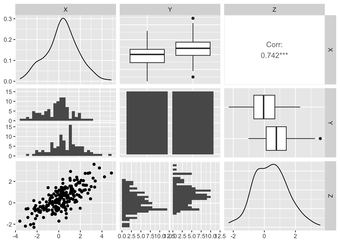
Generate dataset with an effect X, outcome Y, and a confounder Z variables

The random variable Z generates X and Y. Any correlation between X and Y is therefore spurious

Show The Code


import numpy as np
N=100
Z1 = np.random.normal(loc=0,scale=1,size=N)
Z2 = np.random.normal(loc=1,scale=1,size=N)
Z = np.concatenate([Z1,Z2])

import scipy as sc
Y = np.concatenate([sc.stats.bernoulli.rvs(z,size=1) for z in (Z - min(Z)) / (max(Z) - min(Z))])
X = Z + np.random.normal(loc=0,scale=1,size=len(Z))

Show The Code

df <- tibble::tibble(
    X = reticulate::py$X,
    Y = reticulate::py$Y,
    Z = reticulate::py$Z
)
df[['Y']] <- factor(df$Y,levels=c(0,1))

df

# A tibble: 200 × 3
           X Y             Z
   <dbl[1d]> <fct> <dbl[1d]>
 1   -0.861  0       -0.0394
 2   -0.0157 0       -0.649 
 3    0.857  0        0.626 
 4    1.78   0        1.84  
 5   -1.33   0       -0.539 
 6    0.688  0       -1.40  
 7   -0.132  0        0.949 
 8    0.636  0       -0.702 
 9    1.43   0        0.606 
10   -0.276  0       -0.319 
# … with 190 more rows

Show The Code

GGally::ggpairs(df)

Registered S3 method overwritten by 'GGally':
  method from   
  +.gg   ggplot2

`stat_bin()` using `bins = 30`. Pick better value with `binwidth`.
`stat_bin()` using `bins = 30`. Pick better value with `binwidth`.

Employ MCCV: Predict Y from X, Y from Z, Y from X and Z

Show The Code

import pandas as pd
df = pd.DataFrame(data={'X' : X,'Y' : Y,'Z' : Z})
df.index.name = 'pt'

X = df.loc[:,['X']]
Y = df.loc[:,['Y']]
Z = df.loc[:,['Z']]
XZ = df.loc[:,['X','Z']]

Show The Code

import mccv

mccv_YXobj = mccv.mccv(num_bootstraps=200,n_jobs=2)
mccv_YXobj.set_X(X)
mccv_YXobj.set_Y(Y)
mccv_YXobj.run_mccv()

mccv_YZobj = mccv.mccv(num_bootstraps=200,n_jobs=2)
mccv_YZobj.set_X(Z)
mccv_YZobj.set_Y(Y)
mccv_YZobj.run_mccv()

mccv_YXZobj = mccv.mccv(num_bootstraps=200,n_jobs=2)
mccv_YXZobj.set_X(XZ)
mccv_YXZobj.set_Y(Y)
mccv_YXZobj.run_mccv()

Show The Code


f_imp_dfs = dict()
f_imp_dfs['YXobj'] = \
mccv_YXobj.mccv_data['Feature Importance']
f_imp_dfs['YZobj'] = \
mccv_YZobj.mccv_data['Feature Importance']
f_imp_dfs['YXZobj'] = \
mccv_YXZobj.mccv_data['Feature Importance']

Visualize feature importances

Show The Code

library(ggplot2)

f_imp_plot <- function(x,title){
    ggplot(x,aes(feature,importance,color=feature)) +
    geom_boxplot(alpha=0) +
    geom_point(position=position_jitter(width=0.2)) +
    scale_color_manual(values=c("X" = "indianred",
                                "Y" = "skyblue",
                                "Z" = "black",
                                "Intercept" = "gray")) +
    theme_bw() +
    labs(title=title)
}

library(patchwork)
(f_imp_plot( reticulate::py$f_imp_dfs$YXobj,"Y ~ X" ) +
    f_imp_plot( reticulate::py$f_imp_dfs$YZobj,"Y ~ Z" ) ) /
    f_imp_plot( reticulate::py$f_imp_dfs$YXZobj,"Y ~ X + Z" )

Warning in py_to_r.pandas.core.frame.DataFrame(object): index contains
duplicated values: row names not set

Warning in py_to_r.pandas.core.frame.DataFrame(object): index contains
duplicated values: row names not set

Warning in py_to_r.pandas.core.frame.DataFrame(object): index contains
duplicated values: row names not set

Warning in py_to_r.pandas.core.frame.DataFrame(object): index contains
duplicated values: row names not set

Warning in py_to_r.pandas.core.frame.DataFrame(object): index contains
duplicated values: row names not set

Warning in py_to_r.pandas.core.frame.DataFrame(object): index contains
duplicated values: row names not set

Warning in py_to_r.pandas.core.frame.DataFrame(object): index contains
duplicated values: row names not set

Warning in py_to_r.pandas.core.frame.DataFrame(object): index contains
duplicated values: row names not set

Warning in py_to_r.pandas.core.frame.DataFrame(object): index contains
duplicated values: row names not set

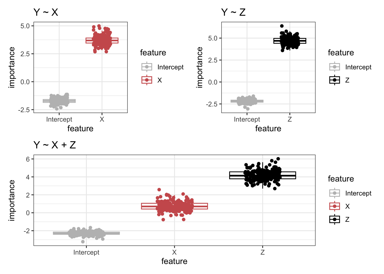
In this example, Z is confounding the relationship between X and Y. The ‘Y ~ X’ model shows that X is very important in predicting Y. However, when Z is included in the model ‘Y ~ X + Z’, you see that Z remains very important but X is no longer important for predicting Y. This toy example had Z causing Y and Z causing X, and any relationship between X and Y was spurious. Therefore, including X and Z as predictors showed only the importance of Z in predicting Y.

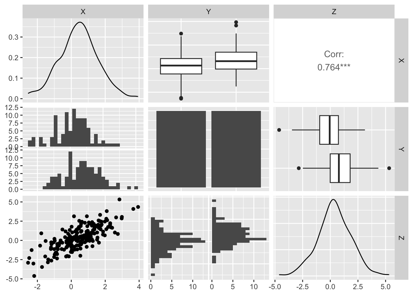
Generate dataset with an effect X, outcome Y, and a mediator Z variables

The random variable X generates Z which generates and Y. Any correlation between X and Y is therefore spurious

Show The Code


import numpy as np
N=100
X1 = np.random.normal(loc=0,scale=1,size=N)
X2 = np.random.normal(loc=1,scale=1,size=N)
X = np.concatenate([X1,X2])

import scipy as sc
Z = X + np.random.normal(loc=0,scale=1,size=len(X))
Y = np.concatenate([sc.stats.bernoulli.rvs(z,size=1) for z in (Z - min(Z)) / (max(Z) - min(Z))])

Show The Code

df <- tibble::tibble(
    X = reticulate::py$X,
    Y = reticulate::py$Y,
    Z = reticulate::py$Z
)
df[['Y']] <- factor(df$Y,levels=c(0,1))

df

# A tibble: 200 × 3
           X Y             Z
   <dbl[1d]> <fct> <dbl[1d]>
 1    -0.566 1        -1.13 
 2     0.728 0         0.519
 3     0.456 0        -0.657
 4    -0.833 0        -0.908
 5    -0.199 1         0.225
 6    -0.241 0        -2.03 
 7     0.322 0        -0.649
 8    -2.55  0        -2.90 
 9     0.350 0        -1.17 
10     0.563 0        -0.117
# … with 190 more rows

Show The Code

GGally::ggpairs(df)

Registered S3 method overwritten by 'GGally':
  method from   
  +.gg   ggplot2

`stat_bin()` using `bins = 30`. Pick better value with `binwidth`.
`stat_bin()` using `bins = 30`. Pick better value with `binwidth`.

Employ MCCV: Predict Y from X, Y from Z, Y from X and Z

Show The Code

import pandas as pd
df = pd.DataFrame(data={'X' : X,'Y' : Y,'Z' : Z})
df.index.name = 'pt'

X = df.loc[:,['X']]
Y = df.loc[:,['Y']]
Z = df.loc[:,['Z']]
XZ = df.loc[:,['X','Z']]

Show The Code

import mccv

mccv_YXobj = mccv.mccv(num_bootstraps=200,n_jobs=2)
mccv_YXobj.set_X(X)
mccv_YXobj.set_Y(Y)
mccv_YXobj.run_mccv()

mccv_YZobj = mccv.mccv(num_bootstraps=200,n_jobs=2)
mccv_YZobj.set_X(Z)
mccv_YZobj.set_Y(Y)
mccv_YZobj.run_mccv()

mccv_YXZobj = mccv.mccv(num_bootstraps=200,n_jobs=2)
mccv_YXZobj.set_X(XZ)
mccv_YXZobj.set_Y(Y)
mccv_YXZobj.run_mccv()

Show The Code


f_imp_dfs = dict()
f_imp_dfs['YXobj'] = \
mccv_YXobj.mccv_data['Feature Importance']
f_imp_dfs['YZobj'] = \
mccv_YZobj.mccv_data['Feature Importance']
f_imp_dfs['YXZobj'] = \
mccv_YXZobj.mccv_data['Feature Importance']

Visualize feature importances

Show The Code

library(ggplot2)

f_imp_plot <- function(x,title){
    ggplot(x,aes(feature,importance,color=feature)) +
    geom_boxplot(alpha=0) +
    geom_point(position=position_jitter(width=0.2)) +
    scale_color_manual(values=c("X" = "indianred",
                                "Y" = "skyblue",
                                "Z" = "black",
                                "Intercept" = "gray")) +
    theme_bw() +
    labs(title=title)
}

library(patchwork)
(f_imp_plot( reticulate::py$f_imp_dfs$YXobj,"Y ~ X" ) +
    f_imp_plot( reticulate::py$f_imp_dfs$YZobj,"Y ~ Z" ) ) /
    f_imp_plot( reticulate::py$f_imp_dfs$YXZobj,"Y ~ X + Z" )

Warning in py_to_r.pandas.core.frame.DataFrame(object): index contains
duplicated values: row names not set

Warning in py_to_r.pandas.core.frame.DataFrame(object): index contains
duplicated values: row names not set

Warning in py_to_r.pandas.core.frame.DataFrame(object): index contains
duplicated values: row names not set

Warning in py_to_r.pandas.core.frame.DataFrame(object): index contains
duplicated values: row names not set

Warning in py_to_r.pandas.core.frame.DataFrame(object): index contains
duplicated values: row names not set

Warning in py_to_r.pandas.core.frame.DataFrame(object): index contains
duplicated values: row names not set

Warning in py_to_r.pandas.core.frame.DataFrame(object): index contains
duplicated values: row names not set

Warning in py_to_r.pandas.core.frame.DataFrame(object): index contains
duplicated values: row names not set

Warning in py_to_r.pandas.core.frame.DataFrame(object): index contains
duplicated values: row names not set

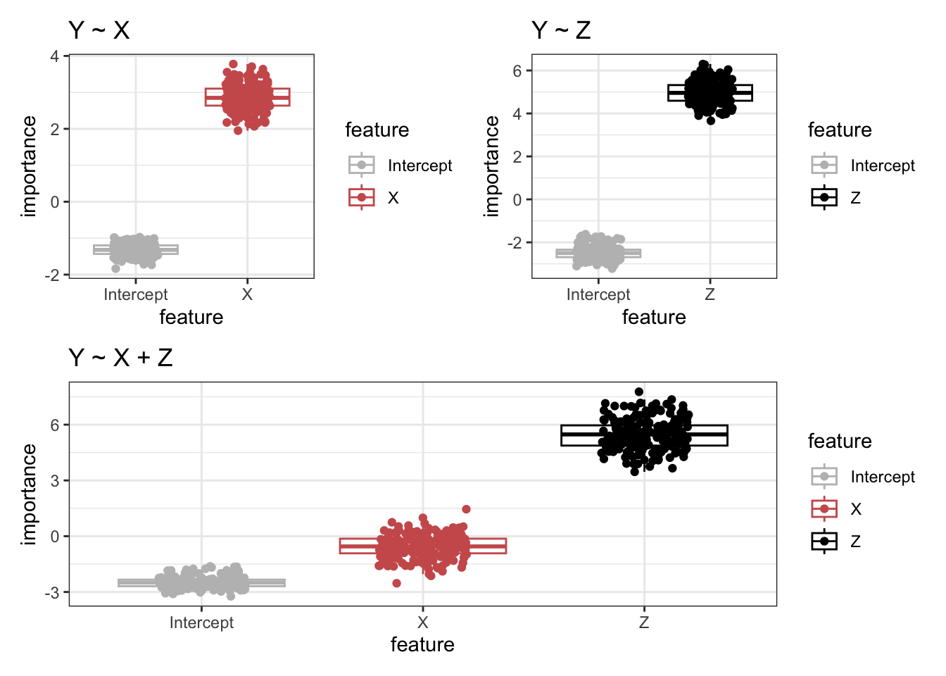
In this example, Z is a mediating relationship between X and Y. The ‘Y ~ X’ model shows that X is very important in predicting Y. However, when Z is included in the model ‘Y ~ X + Z’, you see that Z remains very important but X is no longer important for predicting Y. This toy example had Z causing Y and X relating to Y through Z, and any relationship between X and Y was mediated through Z. Therefore, including X and Z as predictors showed only the importance of Z in predicting Y.