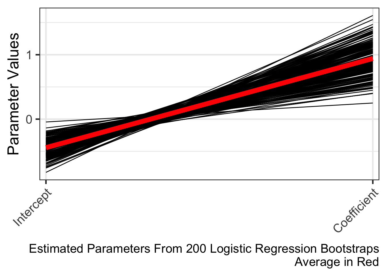
Refitting the model per learned parameters from K-fold cross validation during training is a key step in the Monte Carlo Cross Validation (MCCV) methodology. However, the run_mccv() function that runs the entire MCCV procedure does not return these learned parameters. In this article, the learned parameters are extracted from 10-fold cross validation of a Logistic Regression model. These learned parameters are 200 intercepts and coefficients later refit to the entire training set. Here, we visualize the distribution of the learned parameters to illustrate the learning process.
Show The Code
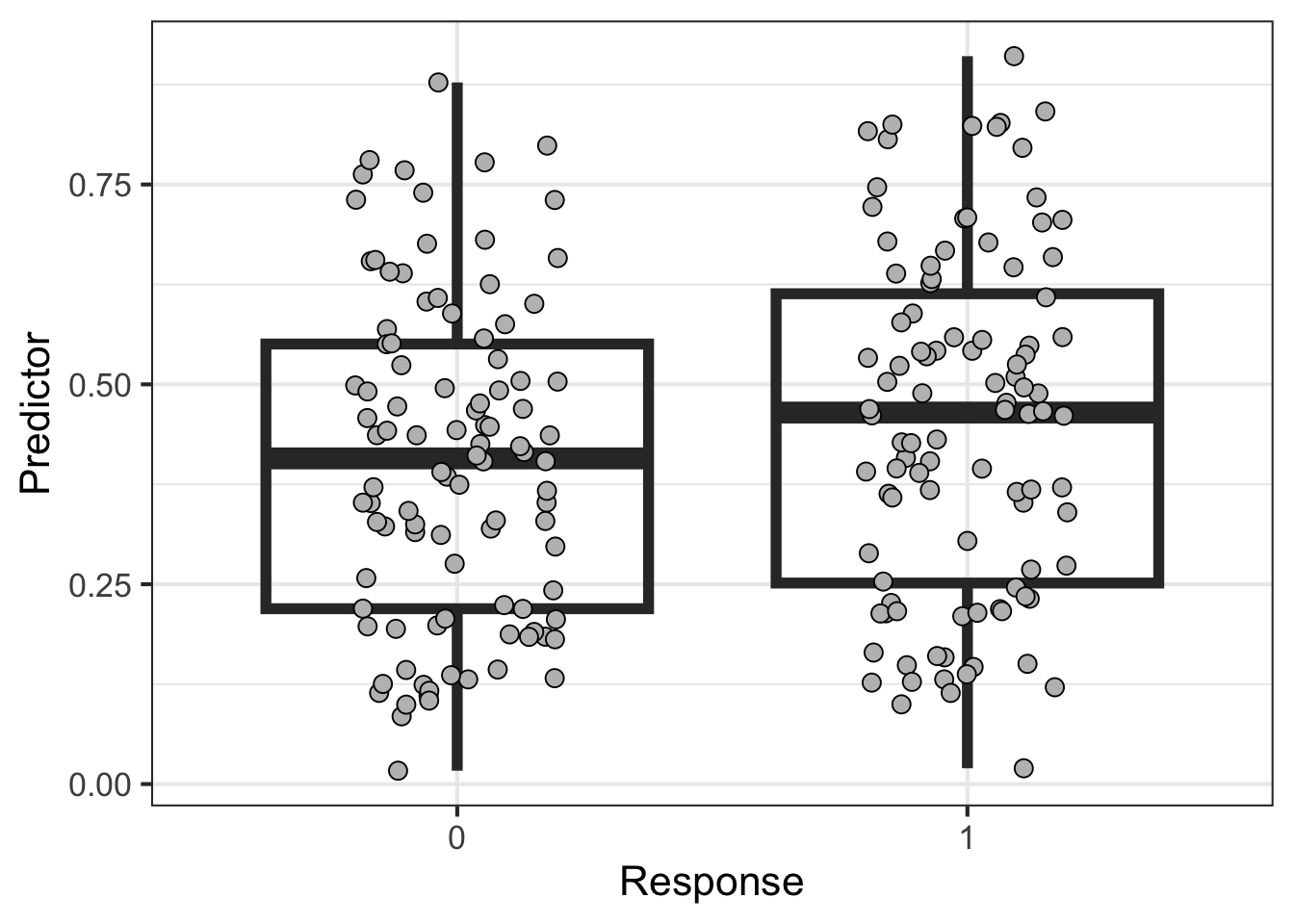
import numpy as npimport scipy as scimport pandas as pdN=100np.random.seed(0)Z1 = np.random.beta(2,3,size=N,)np.random.seed(0)Z2 = np.random.beta(2,2.5,size=N)Z = np.concatenate([Z1,Z2])Y = np.concatenate([np.repeat(0,N),np.repeat(1,N)])df = pd.DataFrame(data={'Y' : Y,'Z' : Z})df.index.name ='pt'
We learned that on average when the predictor is 0, there is a -0.44 log of the odds or 0.64 odds or 0.39 probability to be in the outcome group (Y=1).
On average, there is a 0.94 expected change in the log of the odds or 2.56 odds for a one-unit increase in the predictor. In other words, we expect to see a 72% increase in the odds of being in the outcome group (Y=1) as the predictor increases by one-unit.
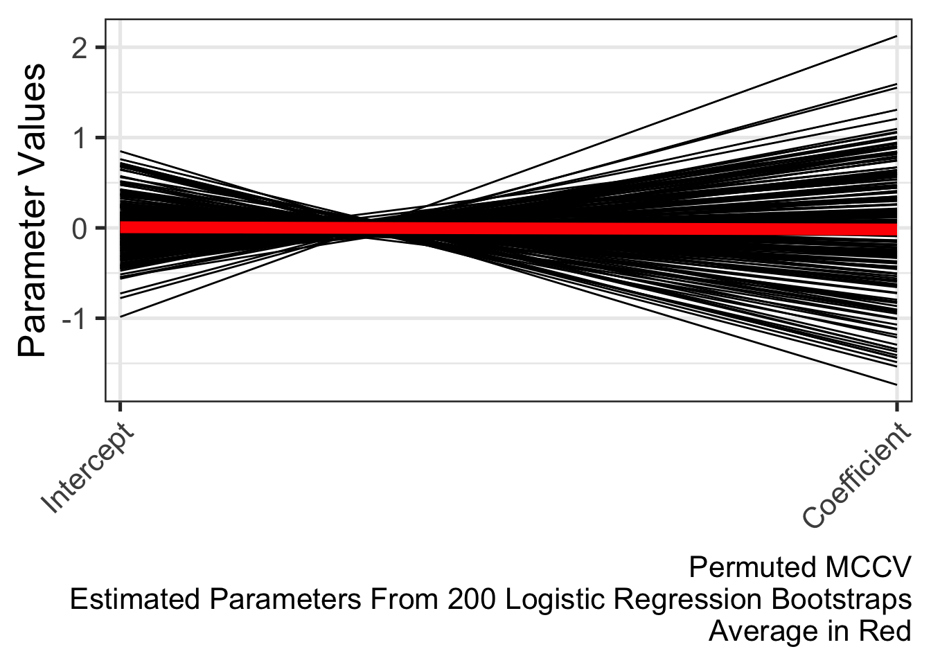
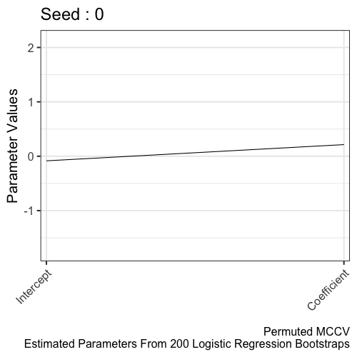
The distribution of parameters from the permuted MCCV provides a null distribution. The alternative hypothesis is learned parameters from MCCV (using the real data) is different from parameters estimated from permuted MCCV (using shuffled data).