Estimating Power

One of the advantages of using MCCV is it’s data-driven approach. Given data, you can answer questions such as:

How predictive is Y from X?
Is a certain cut of the data driving the prediction?
Is there another variable obscuring or influencing the contribution of X in predicting Y?

In this article I want to illustrate another type of question MCCV can address:

How does the prediction of Y by X compare to the prediction by X to a random Y? In other words, what is the power of my data X to predict Y?

I will discuss at the end how the term ‘power’ is used here in comparison to the statistical and more common form of the term. First, I will show two examples showing the power of X to predict Y.

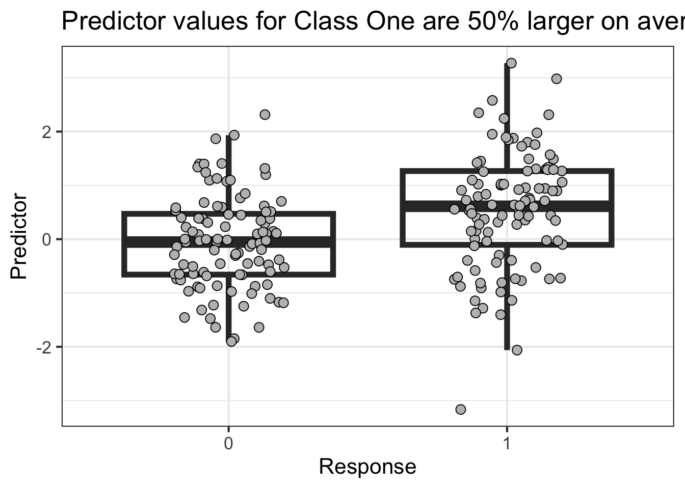
This first example shows low power

Show The Code

import numpy as np
N=100
X1 = np.random.normal(loc=0,scale=1,size=N)
X2 = np.random.normal(loc=0.5,scale=1,size=N)
X = np.concatenate([X1,X2])
Y = np.concatenate([np.repeat(0,N),np.repeat(1,N)])

import pandas as pd
df = pd.DataFrame(data={'Y' : Y,'X' : X})
df.index.name = 'pt'

Show The Code

library(tidyverse)

df <- reticulate::py$df

df[['Y']] <- factor(df$Y,levels=c(0,1))

df %>% 
    ggplot(aes(Y,X)) +
    geom_boxplot(outlier.size = NA,alpha=0,linewidth=2) +
    geom_point(position = position_jitter(width = .2),pch=21,fill='gray',size=3) +
    labs(x = "Response",y="Predictor",title = "Predictor values for Class One are 50% larger on average") +
    theme_bw(base_size = 16)

Show The Code

import mccv

mccv_obj = mccv.mccv(num_bootstraps=200,n_jobs=4)
mccv_obj.set_X(df[['X']])
mccv_obj.set_Y(df[['Y']])
mccv_obj.run_mccv()
mccv_obj.mccv_data['Feature Importance'].insert(
    len(mccv_obj.mccv_data['Feature Importance'].columns),
    'type',
    'real'
)
mccv_obj.mccv_data['Model Learning'].insert(
    len(mccv_obj.mccv_data['Model Learning'].columns),
    'type',
    'real'
)
mccv_obj.mccv_data['Patient Predictions'].insert(
    len(mccv_obj.mccv_data['Patient Predictions'].columns),
    'type',
    'real'
)
mccv_obj.run_permuted_mccv()
mccv_obj.mccv_permuted_data['Feature Importance'].insert(
    len(mccv_obj.mccv_permuted_data['Feature Importance'].columns),
    'type',
    'permuted'
)
mccv_obj.mccv_permuted_data['Model Learning'].insert(
    len(mccv_obj.mccv_permuted_data['Model Learning'].columns),
    'type',
    'permuted'
)
mccv_obj.mccv_permuted_data['Patient Predictions'].insert(
    len(mccv_obj.mccv_permuted_data['Patient Predictions'].columns),
    'type',
    'permuted'
)

fimp_df = \
pd.concat([
    (mccv_obj.mccv_data['Feature Importance'].
    query('feature=="X"').
    reset_index(drop=True)),
    (mccv_obj.mccv_permuted_data['Feature Importance'].
    query('feature=="X"').
    reset_index(drop=True))
])
ppred_df = \
pd.concat([
    (mccv_obj.mccv_data['Patient Predictions'].
    drop('y_pred',axis=1).
    reset_index()),
    (mccv_obj.mccv_permuted_data['Patient Predictions'].
    reset_index().
    drop('y_pred',axis=1))
])
pred_df = \
pd.concat([
    (mccv_obj.mccv_data['Model Learning'].
    reset_index()),
    (mccv_obj.mccv_permuted_data['Model Learning'].
    reset_index())
])

Show The Code

pks <- 
    ks.test(
    reticulate::py$pred_df %>% 
        filter(type=='real') %>% 
        pull(validation_roc_auc),
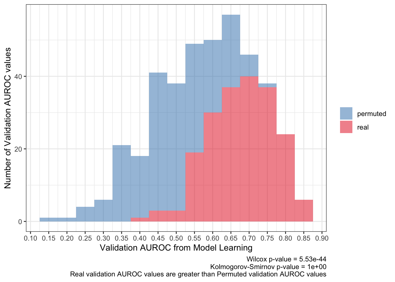
    reticulate::py$pred_df %>% 
        filter(type=='permuted') %>% 
        pull(validation_roc_auc),
    alternative = 'greater'
)[['p.value']]

pwilcox <- 
    wilcox.test(
    reticulate::py$pred_df %>% 
        filter(type=='real') %>% 
        pull(validation_roc_auc),
    reticulate::py$pred_df %>% 
        filter(type=='permuted') %>% 
        pull(validation_roc_auc)
)[['p.value']]

reticulate::py$pred_df %>% 
    ggplot(aes(validation_roc_auc,fill=type)) +
    geom_histogram(aes(y=after_stat(count)),alpha=.5,binwidth = .05) +
    scale_fill_brewer(palette = 'Set1',direction = -1,
                      guide=guide_legend(title=NULL)) +
    theme_bw() +
    scale_x_continuous(
        breaks=seq(0,1,0.05),
    ) +
    labs(x='Validation AUROC from Model Learning',
         y='Number of Validation AUROC values',
         caption=paste0('Wilcox p-value = ',scales::scientific(pwilcox,3),'\n',
                        'Kolmogorov-Smirnov p-value = ',scales::scientific(pks,3),'\n',
                        'Real validation AUROC values are greater than Permuted validation AUROC values'))

Show The Code

pks <- 
    ks.test(
    reticulate::py$fimp_df %>% 
        filter(type=='real') %>% 
        pull(importance),
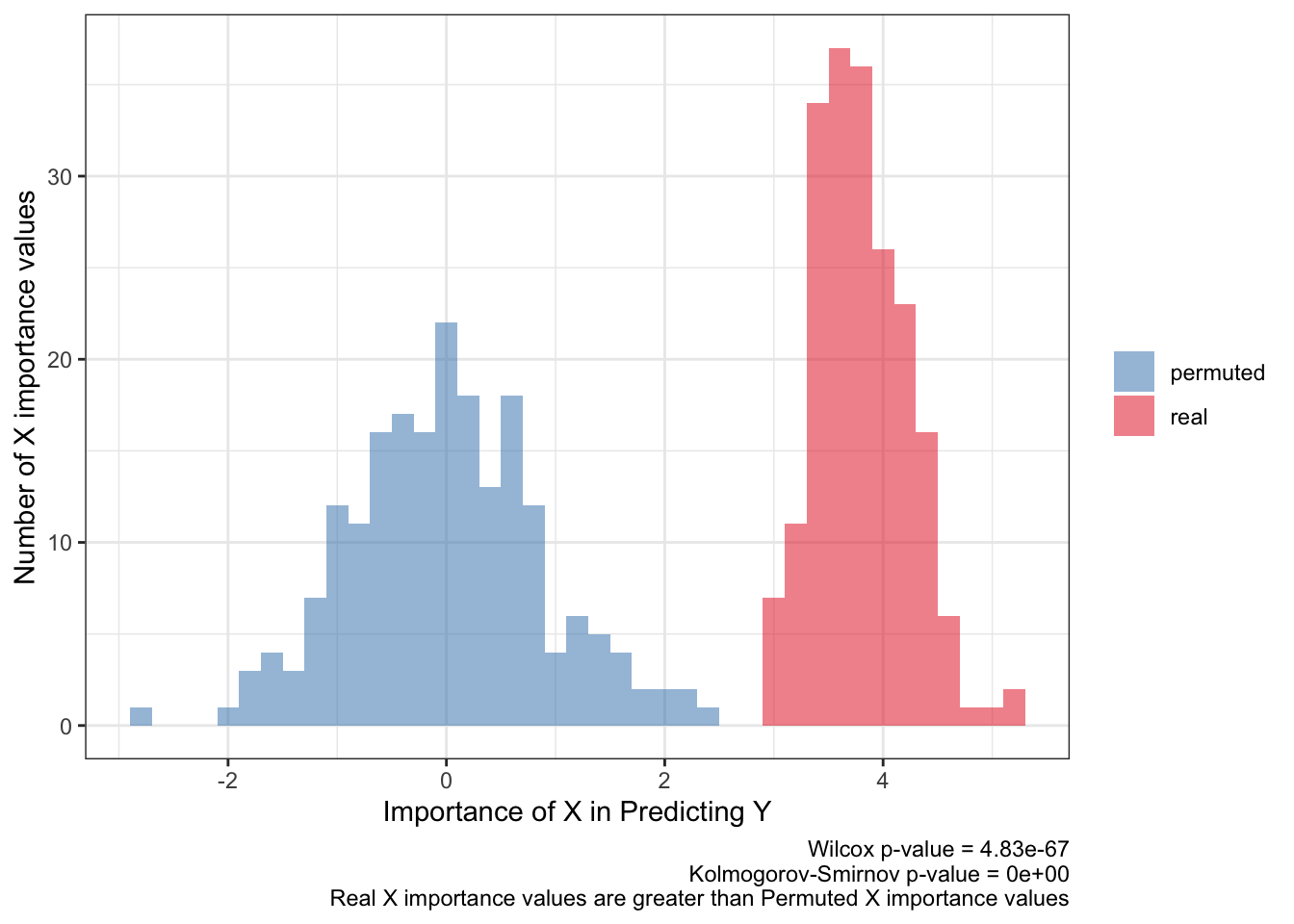
    reticulate::py$fimp_df %>% 
        filter(type=='permuted') %>% 
        pull(importance)
)[['p.value']]

pwilcox <- 
    wilcox.test(
    reticulate::py$fimp_df %>% 
        filter(type=='real') %>% 
        pull(importance),
    reticulate::py$fimp_df %>% 
        filter(type=='permuted') %>% 
        pull(importance)
)[['p.value']]

reticulate::py$fimp_df %>% 
    ggplot(aes(importance,fill=type)) +
    geom_histogram(aes(y=after_stat(count)),alpha=.5,binwidth = .2) +
    scale_fill_brewer(palette = 'Set1',direction = -1,
                      guide=guide_legend(title=NULL)) +
    theme_bw() +
    labs(x='Importance of X in Predicting Y',
         y='Number of X importance values',
         caption=paste0('Wilcox p-value = ',scales::scientific(pwilcox,3),'\n',
                        'Kolmogorov-Smirnov p-value = ',scales::scientific(pks,3),'\n',
                        'Real X importance values are greater than Permuted X importance values'))

Show The Code

pks <- 
    ks.test(
    reticulate::py$ppred_df %>% 
    filter(type=='real' & y_true==1) %>% 
    pull(y_proba),
    reticulate::py$ppred_df %>% 
    filter(type=='permuted' & y_true==1) %>% 
    pull(y_proba)
)[['p.value']]
pwilcox <- 
    wilcox.test(
    reticulate::py$ppred_df %>% 
    filter(type=='real' & y_true==1) %>% 
    pull(y_proba),
    reticulate::py$ppred_df %>% 
    filter(type=='permuted' & y_true==1) %>% 
    pull(y_proba)
)[['p.value']]

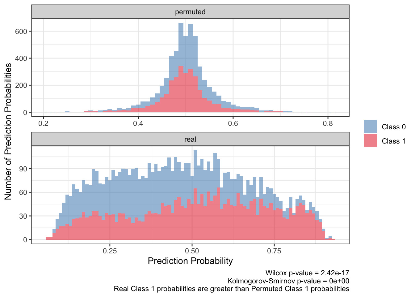
reticulate::py$ppred_df %>% 
    arrange(pt,bootstrap) %>%
    ggplot(aes(y_proba,fill=factor(y_true),group=y_true)) +
    geom_histogram(aes(y=after_stat(count)),alpha=.5,binwidth = .01) +
    scale_fill_brewer(NULL,
                      palette = 'Set1',
                      direction = -1,
                      labels=c("Class 0","Class 1"),
                      guide=guide_legend(title=NULL)) +
    facet_wrap(~type,ncol=1,scales='free') +
    theme_bw() +
    labs(x='Prediction Probability',
         y='Number of Prediction Probabilities',
         caption = paste0('Wilcox p-value = ',scales::scientific(pwilcox,3),'\n',
                          'Kolmogorov-Smirnov p-value = ',scales::scientific(pks,3),'\n',
                        'Real Class 1 probabilities are greater than Permuted Class 1 probabilities'))

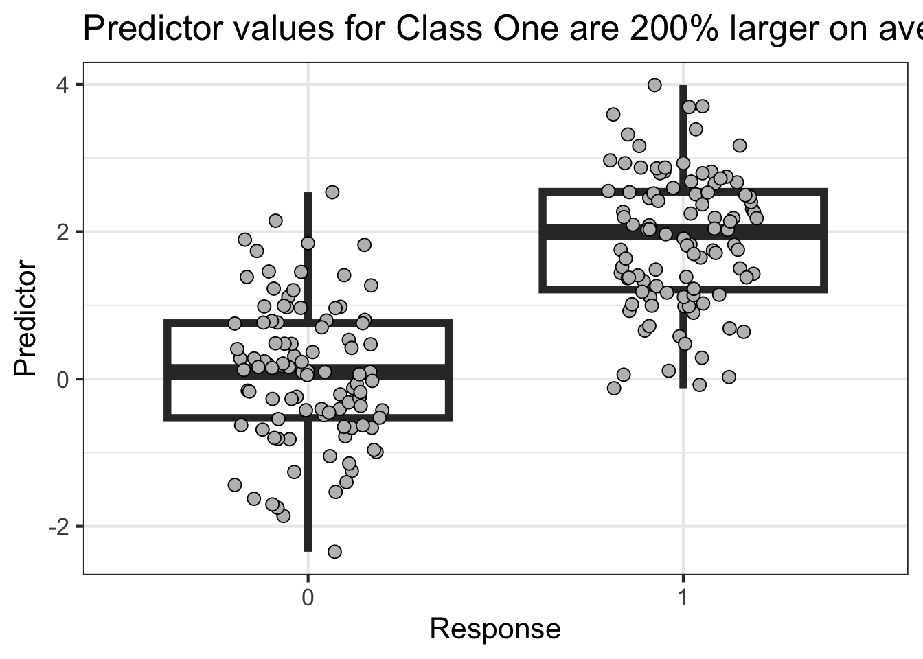
This next example shows high power

Show The Code

import numpy as np
N=100
X1 = np.random.normal(loc=0,scale=1,size=N)
X2 = np.random.normal(loc=2,scale=1,size=N)
X = np.concatenate([X1,X2])
Y = np.concatenate([np.repeat(0,N),np.repeat(1,N)])

import pandas as pd
df = pd.DataFrame(data={'Y' : Y,'X' : X})
df.index.name = 'pt'

Show The Code

library(tidyverse)

df <- reticulate::py$df

df[['Y']] <- factor(df$Y,levels=c(0,1))

df %>% 
    ggplot(aes(Y,X)) +
    geom_boxplot(outlier.size = NA,alpha=0,linewidth=2) +
    geom_point(position = position_jitter(width = .2),pch=21,fill='gray',size=3) +
    labs(x = "Response",y="Predictor",title = "Predictor values for Class One are 200% larger on average") +
    theme_bw(base_size = 16)

Show The Code

import mccv

mccv_obj = mccv.mccv(num_bootstraps=200,n_jobs=4)
mccv_obj.set_X(df[['X']])
mccv_obj.set_Y(df[['Y']])
mccv_obj.run_mccv()
mccv_obj.mccv_data['Feature Importance'].insert(
    len(mccv_obj.mccv_data['Feature Importance'].columns),
    'type',
    'real'
)
mccv_obj.mccv_data['Model Learning'].insert(
    len(mccv_obj.mccv_data['Model Learning'].columns),
    'type',
    'real'
)
mccv_obj.mccv_data['Patient Predictions'].insert(
    len(mccv_obj.mccv_data['Patient Predictions'].columns),
    'type',
    'real'
)
mccv_obj.run_permuted_mccv()
mccv_obj.mccv_permuted_data['Feature Importance'].insert(
    len(mccv_obj.mccv_permuted_data['Feature Importance'].columns),
    'type',
    'permuted'
)
mccv_obj.mccv_permuted_data['Model Learning'].insert(
    len(mccv_obj.mccv_permuted_data['Model Learning'].columns),
    'type',
    'permuted'
)
mccv_obj.mccv_permuted_data['Patient Predictions'].insert(
    len(mccv_obj.mccv_permuted_data['Patient Predictions'].columns),
    'type',
    'permuted'
)

fimp_df = \
pd.concat([
    (mccv_obj.mccv_data['Feature Importance'].
    query('feature=="X"').
    reset_index(drop=True)),
    (mccv_obj.mccv_permuted_data['Feature Importance'].
    query('feature=="X"').
    reset_index(drop=True))
])
ppred_df = \
pd.concat([
    (mccv_obj.mccv_data['Patient Predictions'].
    drop('y_pred',axis=1).
    reset_index()),
    (mccv_obj.mccv_permuted_data['Patient Predictions'].
    reset_index().
    drop('y_pred',axis=1))
])
pred_df = \
pd.concat([
    (mccv_obj.mccv_data['Model Learning'].
    reset_index()),
    (mccv_obj.mccv_permuted_data['Model Learning'].
    reset_index())
])

Show The Code

pks <- 
    ks.test(
    reticulate::py$pred_df %>% 
        filter(type=='real') %>% 
        pull(validation_roc_auc),
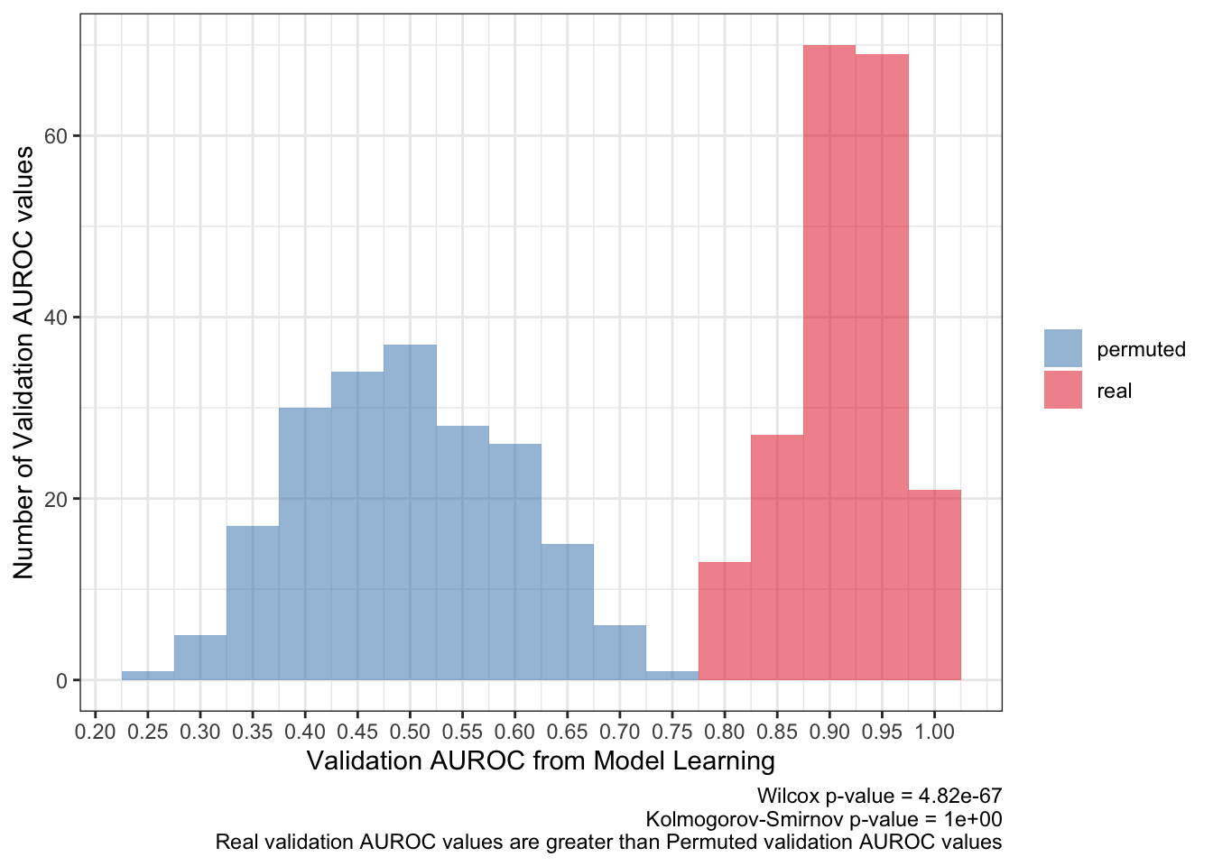
    reticulate::py$pred_df %>% 
        filter(type=='permuted') %>% 
        pull(validation_roc_auc),
    alternative = 'greater'
)[['p.value']]

pwilcox <- 
    wilcox.test(
    reticulate::py$pred_df %>% 
        filter(type=='real') %>% 
        pull(validation_roc_auc),
    reticulate::py$pred_df %>% 
        filter(type=='permuted') %>% 
        pull(validation_roc_auc)
)[['p.value']]

reticulate::py$pred_df %>% 
    ggplot(aes(validation_roc_auc,fill=type)) +
    geom_histogram(aes(y=after_stat(count)),alpha=.5,binwidth = .05) +
    scale_fill_brewer(palette = 'Set1',direction = -1,
                      guide=guide_legend(title=NULL)) +
    theme_bw() +
    scale_x_continuous(
        breaks=seq(0,1,0.05),
    ) +
    labs(x='Validation AUROC from Model Learning',
         y='Number of Validation AUROC values',
         caption=paste0('Wilcox p-value = ',scales::scientific(pwilcox,3),'\n',
                        'Kolmogorov-Smirnov p-value = ',scales::scientific(pks,3),'\n',
                        'Real validation AUROC values are greater than Permuted validation AUROC values'))

Show The Code

pks <- 
    ks.test(
    reticulate::py$fimp_df %>% 
        filter(type=='real') %>% 
        pull(importance),
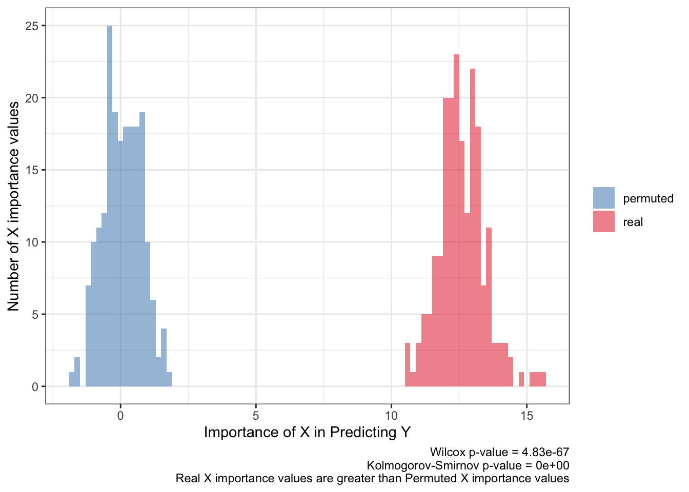
    reticulate::py$fimp_df %>% 
        filter(type=='permuted') %>% 
        pull(importance)
)[['p.value']]

pwilcox <- 
    wilcox.test(
    reticulate::py$fimp_df %>% 
        filter(type=='real') %>% 
        pull(importance),
    reticulate::py$fimp_df %>% 
        filter(type=='permuted') %>% 
        pull(importance)
)[['p.value']]

reticulate::py$fimp_df %>% 
    ggplot(aes(importance,fill=type)) +
    geom_histogram(aes(y=after_stat(count)),alpha=.5,binwidth = .2) +
    scale_fill_brewer(palette = 'Set1',direction = -1,
                      guide=guide_legend(title=NULL)) +
    theme_bw() +
    labs(x='Importance of X in Predicting Y',
         y='Number of X importance values',
         caption=paste0('Wilcox p-value = ',scales::scientific(pwilcox,3),'\n',
                        'Kolmogorov-Smirnov p-value = ',scales::scientific(pks,3),'\n',
                        'Real X importance values are greater than Permuted X importance values'))

Show The Code

pks <- 
    ks.test(
    reticulate::py$ppred_df %>% 
    filter(type=='real' & y_true==1) %>% 
    pull(y_proba),
    reticulate::py$ppred_df %>% 
    filter(type=='permuted' & y_true==1) %>% 
    pull(y_proba)
)[['p.value']]
pwilcox <- 
    wilcox.test(
    reticulate::py$ppred_df %>% 
    filter(type=='real' & y_true==1) %>% 
    pull(y_proba),
    reticulate::py$ppred_df %>% 
    filter(type=='permuted' & y_true==1) %>% 
    pull(y_proba)
)[['p.value']]

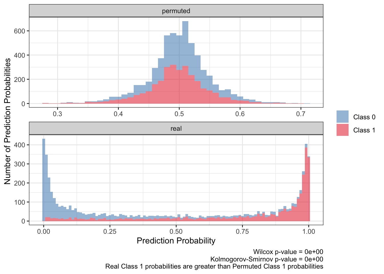
reticulate::py$ppred_df %>% 
    arrange(pt,bootstrap) %>%
    ggplot(aes(y_proba,fill=factor(y_true),group=y_true)) +
    geom_histogram(aes(y=after_stat(count)),alpha=.5,binwidth = .01) +
    scale_fill_brewer(NULL,
                      palette = 'Set1',
                      direction = -1,
                      labels=c("Class 0","Class 1"),
                      guide=guide_legend(title=NULL)) +
    facet_wrap(~type,ncol=1,scales='free') +
    theme_bw() +
    labs(x='Prediction Probability',
         y='Number of Prediction Probabilities',
         caption = paste0('Wilcox p-value = ',scales::scientific(pwilcox,3),'\n',
                          'Kolmogorov-Smirnov p-value = ',scales::scientific(pks,3),'\n',
                        'Real Class 1 probabilities are greater than Permuted Class 1 probabilities'))

These two examples show different metrics for defining a ‘powerful’ prediction. Here, a powerful prediction can only be defined by the combination of different components to describe how and to what degree a predictor X can predict a response Y. These components can come from the model learning process as well as the applying the model on new data i.e. a validation set. Defining a powerful prediction is difficult using only one quantitative metric, like the statistical tests shown in the plot captions. But a few metrics noted here (and probably others I’ve mistakingly overlooked) can accurately define a powerful prediction:

The average AUROC for the validation set should be more than 50%. To be more strict, the 95% confidence interval should be greater than 50% AUROC.
The importance value (beta coefficient for logistic regression) of X for predicting Y should be above the null association i.e. 0 and should barely overlap the importance values for a shuffled response. Statistical tests will probably produce a false positive by showing a small p-value, like here, so they shouldn’t be the metric in defining a powerful prediction.
There seems to be at least two takeaways from the distributions of the prediction probabilities. First, the distribution of the real predicted probabilities for class 1 need to be greater than that for class 0. Also the distribution of real, class 1 predicted probabilities need to be greater than the distribution of permuted, class 1 predicted probabilities.

I used a combination of the metrics referenced above in the papers published using MCCV. This article’s toy examples illustrate why these metrics are sensible for defining the power of a prediction given the data.